In this instalment of Microsoft Excel tips, we discuss how to find specific values in a series of data

Today's Excel tip for those less experienced users is how to find the Minimum, Maximum, Average, Largest and Smallest numbers from a series of data.

Sometimes we want to know what was the highest (or lowest value) of the NZ$ over a time period, or what is the average 2 year fixed mortgage rate across all the lending institutions. These questions can be answered simply using Excel.

Many of the tips you may know, but there may also be some ideas here that you could find useful that you did not know about.

We encourage you to use the comment section below to add in your own tips.

---------------------------------------------------------------------------------------------

The examples below uses the following set of data, which just happens to be the 2-year swap rates from 7 January to 15 February 2013.

2.83%
2.82%
2.81%
2.81%
2.81%
2.84%
2.84%
2.86%
2.85%
2.82%
2.81%
2.81%
2.87%
2.85%
2.85%
2.83%
2.92%
2.95%
2.92%
2.93%
2.95%
3.00%
2.97%
2.93%
2.94%
2.90%
2.96%
2.99%
3.01%

Finding the Maximum value (MAX)

Imagine you create a new spreadsheet and insert these numbers starting in column A row 1 - the data should finish in cell A29.

To calculate the highest 2-year swap rate you would type the following formula into cell A30: =MAX(A1:A29).

The number returned should be 3.01%.

Finding the Minimum value (MIN)

Using the data and same range as above for finding the maximum, replace the word MAX with the word MIN, the number returned should be 2.81%.

What if we wanted to find the average, or third largest, or third smallest numbers in our series?

AVERAGE

To find the average of the numbers in our series we use the AVERAGE function. Type the formula =AVERAGE(A1:A29) into cell A30 and the result you should get is 2.89%. You use MEDIAN and MODE is a similar way. (Median is the middle value, Mode is the most common value.)

LARGE

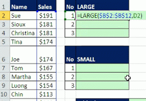
To find the third largest number we would enter the formula =LARGE(A1:A29,3) in cell A30 - the number three is entered in the formula because we are looking for the third largest number in the series range. The number that is returned is 2.99%. If we wanted to find the 10 largest number we would replace the number 3 with the number 10.

SMALL

To find the third smallest number we would enter the formula =SMALL(A1:A29,3) - the number three is entered in the formula because we are looking for the third smallest number in the series range. The number that is returned is 2.81%.

You can also use the Large and Small functions instead of the min and max by simply putting the number 1 in the formula (instead of the number 3 in our example).

---------------------------------------------------------------------------------------------

We encourage you to use the comment section below to add in your own tips about this function. Or ask a question ...

The following video deals with how to use the Large and Small formulae, and goes into much more depth on how an expert user can take advantage of them. Well worth a watch.